Change of Variables in Multiple Integrals

5.7 Change of Variables in Multiple Integrals

Learning Objectives

  • 5.7.1 Determine the image of a region under a given transformation of variables.
  • 5.7.2 Compute the Jacobian of a given transformation.
  • 5.7.3 Evaluate a double integral using a change of variables.
  • 5.7.4 Evaluate a triple integral using a change of variables.

Recall from Substitution Rule the method of integration by substitution. When evaluating an integral such as ∫23x(x2−4)5dx,∫23x(x2−4)5dx, we substitute u=g(x)=x2−4.u=g(x)=x2−4. Then du=2xdxdu=2xdx or xdx=12duxdx=12du and the limits change to u=g(2)=22−4=0u=g(2)=22−4=0 and u=g(3)=9−4=5.u=g(3)=9−4=5. Thus the integral becomes ∫0512u5du∫0512u5du and this integral is much simpler to evaluate. In other words, when solving integration problems, we make appropriate substitutions to obtain an integral that becomes much simpler than the original integral.

We also used this idea when we transformed double integrals in rectangular coordinates to polar coordinates and transformed triple integrals in rectangular coordinates to cylindrical or spherical coordinates to make the computations simpler. More generally,

∫abf(x)dx=∫cdf(g(u))g′(u)du,∫abf(x)dx=∫cdf(g(u))g′(u)du,

Where x=g(u),dx=g′(u)du,x=g(u),dx=g′(u)du, and u=cu=c and u=du=d satisfy c=g-1(a)c=g-1(a) and d=g-1(b).d=g-1(b).

A similar result occurs in double integrals when we substitute x=h(r,θ)=rcosθ,x=h(r,θ)=rcosθ, y=g(r,θ)=rsinθ,y=g(r,θ)=rsinθ, and dA=dxdy=rdrdθ.dA=dxdy=rdrdθ. Then we get

∬Rf(x,y)dA=∬Sf(rcosθ,rsinθ)rdrdθ∬Rf(x,y)dA=∬Sf(rcosθ,rsinθ)rdrdθ

where the domain RR is replaced by the domain SS in polar coordinates. Generally, the function that we use to change the variables to make the integration simpler is called a transformation or mapping.

Planar Transformations

A planar transformation TT is a function that transforms a region GG in one plane into a region RR in another plane by a change of variables. Both GG and RR are subsets of ℝ2.ℝ2. For example, Figure 5.71 shows a region GG in the uv-planeuv-plane transformed into a region RR in the xy-planexy-plane by the change of variables x=g(u,v)x=g(u,v) and y=h(u,v),y=h(u,v), or sometimes we write x=x(u,v)x=x(u,v) and y=y(u,v).y=y(u,v). We shall typically assume that each of these functions has continuous first partial derivatives, which means gu,gv,hu,gu,gv,hu, and hvhv exist and are also continuous. The need for this requirement will become clear soon.

On the left-hand side of this figure, there is a region G with point (u, v) given in the Cartesian u v-plane. Then there is an arrow from this graph to the right-hand side of the figure marked with x = g(u, v) and y = h(u, v). On the right-hand side of this figure there is a region R with point (x, y) given in the Cartesian xy- plane.
Figure 5.71 The transformation of a region GG in the uv-planeuv-plane into a region RR in the xy-plane.xy-plane.

Definition

A transformation T:G→R,T:G→R, defined as T(u,v)=(x,y),T(u,v)=(x,y), is said to be a one-to-one transformation if no two points map to the same image point.

To show that TT is a one-to-one transformation, we assume T(u1,v1)=T(u2,v2)T(u1,v1)=T(u2,v2) and show that as a consequence we obtain (u1,v1)=(u2,v2).(u1,v1)=(u2,v2). If the transformation TT is one-to-one in the domain G,G, then the inverse T−1T−1 exists with the domain RR such that T−1∘TT−1∘T and T∘T−1T∘T−1 are identity functions.

Figure 5.71 shows the mapping T(u,v)=(x,y)T(u,v)=(x,y) where xx and yy are related to uu and vv by the equations x=g(u,v)x=g(u,v) and y=h(u,v).y=h(u,v). The region GG is the domain of TT and the region RR is the range of T,T, also known as the image of GG under the transformation T.T.

Example 5.65

Determining How the Transformation Works

Suppose a transformation TT is defined as T(r,θ)=(x,y)T(r,θ)=(x,y) where x=rcosθ,y=rsinθ.x=rcosθ,y=rsinθ. Find the image of the polar rectangle G={(r,θ)|0<r≤1,0≤θ≤π/2}G={(r,θ)|0<r≤1,0≤θ≤π/2} in the rθ-planerθ-plane to a region RR in the xy-plane.xy-plane. Show that TT is a one-to-one transformation in GG and find T−1(x,y).T−1(x,y).

Solution

Since rr varies from 0 to 1 in the rθ-plane,rθ-plane, we have a circular disc of radius 0 to 1 in the xy-plane.xy-plane. Because θθ varies from 0 to π/2π/2 in the rθ-plane,rθ-plane, we end up getting a quarter circle of radius 11 in the first quadrant of the xy-planexy-plane (Figure 5.72). Hence RR is a quarter circle bounded by x2+y2=1x2+y2=1 in the first quadrant.

On the left-hand side of this figure, there is a rectangle G with a marked subrectangle given in the first quadrant of the Cartesian r theta-plane. Then there is an arrow from this graph to the right-hand side of the figure marked with x = r cos theta and y = r sin theta. On the right-hand side of this figure there is a quarter circle R with a marked subannulus (analogous to the rectangle in the other graph) given in the Cartesian x y-plane.
Figure 5.72 A rectangle in the rθ-planerθ-plane is mapped into a quarter circle in the xy-plane.xy-plane.

In order to show that TT is a one-to-one transformation, assume T(r1,θ1)=T(r2,θ2)T(r1,θ1)=T(r2,θ2) and show as a consequence that (r1,θ1)=(r2,θ2).(r1,θ1)=(r2,θ2). In this case, we have

T ( r 1 , θ 1 ) = T ( r 2 , θ 2 ) , ( x 1 , y 1 ) = ( x 2 , y 2 ) , ( r 1 cos θ 1 , r 1 sin θ 1 ) = ( r 2 cos θ 2 , r 2 sin θ 2 ) , r 1 cos θ 1 = r 2 cos θ 2 r 1 sin θ 1 = r 2 sin θ 2 T ( r 1 , θ 1 ) = T ( r 2 , θ 2 ) , ( x 1 , y 1 ) = ( x 2 , y 2 ) , ( r 1 cos θ 1 , r 1 sin θ 1 ) = ( r 2 cos θ 2 , r 2 sin θ 2 ) , r 1 cos θ 1 = r 2 cos θ 2 r 1 sin θ 1 = r 2 sin θ 2

Dividing, we obtain

r 1 cos θ 1 r 1 sin θ 1 = r 2 cos θ 2 r 2 sin θ 2 cos θ 1 sin θ 1 = cos θ 2 sin θ 2 cot θ 1 = cot θ 2 θ 1 = θ 2 r 1 cos θ 1 r 1 sin θ 1 = r 2 cos θ 2 r 2 sin θ 2 cos θ 1 sin θ 1 = cos θ 2 sin θ 2 cot θ 1 = cot θ 2 θ 1 = θ 2

since the cotangent function is one-one function in the interval 0≤θ≤π/2.0≤θ≤π/2. Also, since 0<r≤1,0<r≤1, we have r1=r2,θ1=θ2.r1=r2,θ1=θ2. Therefore, (r1,θ1)=(r2,θ2)(r1,θ1)=(r2,θ2) and TT is a one-to-one transformation from GG into R.R.

To find T−1(x,y)T−1(x,y) solve for r,θr,θ in terms of x,y.x,y. We already know that r2=x2+y2r2=x2+y2 and tanθ=yx.tanθ=yx. Thus T−1(x,y)=(r,θ)T−1(x,y)=(r,θ) is defined as r=x2+y2r=x2+y2 and θ=tan−1(yx).θ=tan−1(yx).

Example 5.66

Finding the Image under TT

Let the transformation TT be defined by T(u,v)=(x,y)T(u,v)=(x,y) where x=u2−v2x=u2−v2 and y=uv.y=uv. Find the image of the triangle in the uv-planeuv-plane with vertices (0,0),(0,1),(0,0),(0,1), and (1,1).(1,1).

Solution

The triangle and its image are shown in Figure 5.73. To understand how the sides of the triangle transform, call the side that joins (0,0)(0,0) and (0,1)(0,1) side A,A, the side that joins (0,0)(0,0) and (1,1)(1,1) side B,B, and the side that joins (1,1)(1,1) and (0,1)(0,1) side C.C.

On the left-hand side of this figure, there is a triangular region given in the Cartesian uv-plane with boundaries A, B, and C represented by the v axis, the line u = v, and the line v = 1, respectively. Then there is an arrow from this graph to the right-hand side of the figure marked with x = u squared minus v squared and y = u v. On the right-hand side of this figure there is a complex region given in the Cartesian x y-plane with boundaries A’, B’, and C’ given by the x axis, y axis, and a line curving from (negative 1, 0) through (0, 1), namely x = y squared minus 1, respectively.
Figure 5.73 A triangular region in the uv-planeuv-plane is transformed into an image in the xy-plane.xy-plane.

For the side A:u=0,0≤v≤1A:u=0,0≤v≤1 transforms to x=−v2,y=0x=−v2,y=0 so this is the side A′A′ that joins (−1,0)(−1,0) and (0,0).(0,0).

For the side B:u=v,0≤u≤1B:u=v,0≤u≤1 transforms to x=0,y=u2x=0,y=u2 so this is the side B′B′ that joins (0,0)(0,0) and (0,1).(0,1).

For the side C:0≤u≤1,v=1C:0≤u≤1,v=1 transforms to x=u2−1,y=ux=u2−1,y=u (hence x=y2−1)x=y2−1) so this is the side C′C′ that makes the upper half of the parabolic arc joining (−1,0)(−1,0) and (0,1).(0,1).

All the points in the entire region of the triangle in the uv-planeuv-plane are mapped inside the parabolic region in the xy-plane.xy-plane.

Checkpoint 5.43

Let a transformation TT be defined as T(u,v)=(x,y)T(u,v)=(x,y) where x=u+v,y=3v.x=u+v,y=3v. Find the image of the rectangle G={(u,v):0≤u≤1,0≤v≤2}G={(u,v):0≤u≤1,0≤v≤2} from the uv-planeuv-plane after the transformation into a region RR in the xy-plane.xy-plane. Show that TT is a one-to-one transformation and find T−1(x,y).T−1(x,y).

Jacobians

Recall that we mentioned near the beginning of this section that each of the component functions must have continuous first partial derivatives, which means that gu,gv,hu,gu,gv,hu, and hvhv exist and are also continuous. A transformation that has this property is called a C1C1 transformation (here CC denotes continuous). Let T(u,v)=(g(u,v),h(u,v)),T(u,v)=(g(u,v),h(u,v)), where x=g(u,v)x=g(u,v) and y=h(u,v),y=h(u,v), be a one-to-one C1C1 transformation. We want to see how it transforms a small rectangular region S,S, ΔuΔu units by ΔvΔv units, in the uv-planeuv-plane (see the following figure).

On the left-hand side of this figure, there is a region S with lower right corner point (u sub 0, v sub 0), height Delta v, and length Delta u given in the Cartesian u v-plane. Then there is an arrow from this graph to the right-hand side of the figure marked with T. On the right-hand side of this figure there is a region R with point (x sub 0, y sub 0) given in the Cartesian x y-plane with sides r(u, v sub 0) along the bottom and r(u sub 0, v) along the left.
Figure 5.74 A small rectangle SS in the uv-planeuv-plane is transformed into a region RR in the xy-plane.xy-plane.

Since x=g(u,v)x=g(u,v) and y=h(u,v),y=h(u,v), we have the position vector r(u,v)=g(u,v)i+h(u,v)jr(u,v)=g(u,v)i+h(u,v)j of the image of the point (u,v).(u,v). Suppose that (u0,v0)(u0,v0) is the coordinate of the point at the lower left corner that mapped to (x0,y0)=T(u0,v0).(x0,y0)=T(u0,v0). The line v=v0v=v0 maps to the image curve with vector function r(u,v0),r(u,v0), and the tangent vector at (x0,y0)(x0,y0) to the image curve is

ru=gu(u0,v0)i+hu(u0,v0)j=∂x∂ui+∂y∂uj.ru=gu(u0,v0)i+hu(u0,v0)j=∂x∂ui+∂y∂uj.

Similarly, the line u=u0u=u0 maps to the image curve with vector function r(u0,v),r(u0,v), and the tangent vector at (x0,y0)(x0,y0) to the image curve is

rv=gv(u0,v0)i+hv(u0,v0)j=∂x∂vi+∂y∂vj.rv=gv(u0,v0)i+hv(u0,v0)j=∂x∂vi+∂y∂vj.

Now, note that

ru=limΔu→0r(u0+Δu,v0)−r(u0,v0)Δusor(u0+Δu,v0)−r(u0,v0)≈Δuru.ru=limΔu→0r(u0+Δu,v0)−r(u0,v0)Δusor(u0+Δu,v0)−r(u0,v0)≈Δuru.

Similarly,

rv=limΔv→0r(u0,v0+Δv)−r(u0,v0)Δvsor(u0,v0+Δv)−r(u0,v0)≈Δvrv.rv=limΔv→0r(u0,v0+Δv)−r(u0,v0)Δvsor(u0,v0+Δv)−r(u0,v0)≈Δvrv.

This allows us to estimate the area ΔAΔA of the image RR by finding the area of the parallelogram formed by the sides ΔvrvΔvrv and Δuru.Δuru. By using the cross product of these two vectors by adding the k component as 0,0, the area ΔAΔA of the image RR (refer to The Cross Product) is approximately ||Δuru×Δvrv||=||ru×rv||ΔuΔv.||Δuru×Δvrv||=||ru×rv||ΔuΔv. In determinant form, the cross product is

ru×rv=|ijk∂x∂u∂y∂u0∂x∂v∂y∂v0|=|∂x∂u∂y∂u∂x∂v∂y∂v|k=(∂x∂u∂y∂v−∂x∂v∂y∂u)k.ru×rv=|ijk∂x∂u∂y∂u0∂x∂v∂y∂v0|=|∂x∂u∂y∂u∂x∂v∂y∂v|k=(∂x∂u∂y∂v−∂x∂v∂y∂u)k.

Since ||k||=1,||k||=1, we have ΔA≈||ru×rv||ΔuΔv=(∂x∂u∂y∂v−∂x∂v∂y∂u)ΔuΔv.ΔA≈||ru×rv||ΔuΔv=(∂x∂u∂y∂v−∂x∂v∂y∂u)ΔuΔv.

Definition

The Jacobian of the C1C1 transformation T(u,v)=(g(u,v),h(u,v))T(u,v)=(g(u,v),h(u,v)) is denoted by J(u,v)J(u,v) and is defined by the 2×22×2 determinant

J(u,v)=|∂(x,y)∂(u,v)|=|∂x∂u∂y∂u∂x∂v∂y∂v|=(∂x∂u∂y∂v−∂x∂v∂y∂u).J(u,v)=|∂(x,y)∂(u,v)|=|∂x∂u∂y∂u∂x∂v∂y∂v|=(∂x∂u∂y∂v−∂x∂v∂y∂u).

Using the definition, we have

ΔA≈J(u,v)ΔuΔv=|∂(x,y)∂(u,v)|ΔuΔv.ΔA≈J(u,v)ΔuΔv=|∂(x,y)∂(u,v)|ΔuΔv.

Note that the Jacobian is frequently denoted simply by

J(u,v)=∂(x,y)∂(u,v).J(u,v)=∂(x,y)∂(u,v).

Note also that

|∂x∂u∂y∂u∂x∂v∂y∂v|=(∂x∂u∂y∂v−∂x∂v∂y∂u)=|∂x∂u∂x∂v∂y∂u∂y∂v|.|∂x∂u∂y∂u∂x∂v∂y∂v|=(∂x∂u∂y∂v−∂x∂v∂y∂u)=|∂x∂u∂x∂v∂y∂u∂y∂v|.

Hence the notation J(u,v)=∂(x,y)∂(u,v)J(u,v)=∂(x,y)∂(u,v) suggests that we can write the Jacobian determinant with partials of xx in the first row and partials of yy in the second row.

Example 5.67

Finding the Jacobian

Find the Jacobian of the transformation given in Example 5.65.

Solution

The transformation in the example is T(r,θ)=(rcosθ,rsinθ)T(r,θ)=(rcosθ,rsinθ) where x=rcosθx=rcosθ and y=rsinθ.y=rsinθ. Thus the Jacobian is

J ( r , θ ) = ∂ ( x , y ) ∂ ( r , θ ) = | ∂ x ∂ r ∂ x ∂ θ ∂ y ∂ r ∂ y ∂ θ | = | cos θ − r sin θ sin θ r cos θ | = r cos 2 θ + r sin 2 θ = r ( cos 2 θ + sin 2 θ ) = r . J ( r , θ ) = ∂ ( x , y ) ∂ ( r , θ ) = | ∂ x ∂ r ∂ x ∂ θ ∂ y ∂ r ∂ y ∂ θ | = | cos θ − r sin θ sin θ r cos θ | = r cos 2 θ + r sin 2 θ = r ( cos 2 θ + sin 2 θ ) = r .

Example 5.68

Finding the Jacobian

Find the Jacobian of the transformation given in Example 5.66.

Solution

The transformation in the example is T(u,v)=(u2−v2,uv)T(u,v)=(u2−v2,uv) where x=u2−v2x=u2−v2 and y=uv.y=uv. Thus the Jacobian is

J ( u , v ) = ∂ ( x , y ) ∂ ( u , v ) = | ∂ x ∂ u ∂ x ∂ v ∂ y ∂ u ∂ y ∂ v | = | 2 u v − 2 v u | = 2 u 2 + 2 v 2 . J ( u , v ) = ∂ ( x , y ) ∂ ( u , v ) = | ∂ x ∂ u ∂ x ∂ v ∂ y ∂ u ∂ y ∂ v | = | 2 u v − 2 v u | = 2 u 2 + 2 v 2 .

Checkpoint 5.44

Find the Jacobian of the transformation: T(u,v)=(u+v,2v).T(u,v)=(u+v,2v).

Change of Variables for Double Integrals

We have already seen that, under the change of variables T(u,v)=(x,y)T(u,v)=(x,y) where x=g(u,v)x=g(u,v) and y=h(u,v),y=h(u,v), a small region ΔAΔA in the xy-planexy-plane is related to the area formed by the product ΔuΔvΔuΔv in the uv-planeuv-plane by the approximation

ΔA≈J(u,v)Δu,Δv.ΔA≈J(u,v)Δu,Δv.

Now let’s go back to the definition of double integral for a minute:

∬Rf(x,y)dA=limm,n→∞∑i=1m∑j=1nf(xij,yij)ΔA.∬Rf(x,y)dA=limm,n→∞∑i=1m∑j=1nf(xij,yij)ΔA.

Referring to Figure 5.75, observe that we divided the region SS in the uv-planeuv-plane into small subrectangles SijSij and we let the subrectangles RijRij in the xy-planexy-plane be the images of SijSij under the transformation T(u,v)=(x,y).T(u,v)=(x,y).

On the left-hand side of this figure, there is a rectangle S with an inscribed red oval and a subrectangle with lower right corner point (u sub ij, v sub ij), height Delta v, and length Delta u given in the Cartesian u v-plane. Then there is an arrow from this graph to the right-hand side of the figure marked with T. On the right-hand side of this figure there is a region R with inscribed (deformed) red oval and a subrectangle R sub ij with corner point (x sub ij, y sub ij) given in the Cartesian x y-plane. The subrectangle is blown up and shown with vectors pointing along the edge from the corner point.
Figure 5.75 The subrectangles SijSij in the uv-planeuv-plane transform into subrectangles RijRij in the xy-plane.xy-plane.

Then the double integral becomes

∬Rf(x,y)dA=limm,n→∞∑i=1m∑j=1nf(xij,yij)ΔA=limm,n→∞∑i=1m∑j=1nf(g(uij,vij),h(uij,vij))|J(uij,vij)|ΔuΔv.∬Rf(x,y)dA=limm,n→∞∑i=1m∑j=1nf(xij,yij)ΔA=limm,n→∞∑i=1m∑j=1nf(g(uij,vij),h(uij,vij))|J(uij,vij)|ΔuΔv.

Notice this is exactly the double Riemann sum for the integral

∬Sf(g(u,v),h(u,v))|∂(x,y)∂(u,v)|dudv.∬Sf(g(u,v),h(u,v))|∂(x,y)∂(u,v)|dudv.

Theorem 5.14

Change of Variables for Double Integrals

Let T(u,v)=(x,y)T(u,v)=(x,y) where x=g(u,v)x=g(u,v) and y=h(u,v)y=h(u,v) be a one-to-one C1C1 transformation, with a nonzero Jacobian on the interior of the region SS in the uv-plane;uv-plane; it maps SS into the region RR in the xy-plane.xy-plane. If ff is continuous on R,R, then

∬Rf(x,y)dA=∬Sf(g(u,v),h(u,v))|∂(x,y)∂(u,v)|dudv.∬Rf(x,y)dA=∬Sf(g(u,v),h(u,v))|∂(x,y)∂(u,v)|dudv.

With this theorem for double integrals, we can change the variables from (x,y)(x,y) to (u,v)(u,v) in a double integral simply by replacing

dA=dxdy=|∂(x,y)∂(u,v)|dudvdA=dxdy=|∂(x,y)∂(u,v)|dudv

when we use the substitutions x=g(u,v)x=g(u,v) and y=h(u,v)y=h(u,v) and then change the limits of integration accordingly. This change of variables often makes any computations much simpler.

Example 5.69

Changing Variables from Rectangular to Polar Coordinates

Consider the integral

∫02∫02x−x2x2+y2dydx.∫02∫02x−x2x2+y2dydx.

Use the change of variables x=rcosθx=rcosθ and y=rsinθ,y=rsinθ, and find the resulting integral.

Solution

First we need to find the region of integration. This region is bounded below by y=0y=0 and above by y=2x−x2y=2x−x2 (see the following figure).

A semicircle in the first quadrant of the xy plane with radius 1 and center (1, 0). The equation for this curve is given as y = the square root of (2x minus x squared)
Figure 5.76 Changing a region from rectangular to polar coordinates.

Squaring and collecting terms, we find that the region is the upper half of the circle x2+y2−2x=0,x2+y2−2x=0, that is, y2+(x−1)2=1.y2+(x−1)2=1. In polar coordinates, the circle is r=2cosθr=2cosθ so the region of integration in polar coordinates is bounded by 0≤r≤2 cosθ0≤r≤2 cosθ and 0≤θ≤π2.0≤θ≤π2.

The Jacobian is J(r,θ)=r,J(r,θ)=r, as shown in Example 5.67. Since r≥0,r≥0, we have |J(r,θ)|=r.|J(r,θ)|=r.

The integrand x2+y2x2+y2 changes to rr in polar coordinates, so the double iterated integral is

∫ 0 2 ∫ 0 2 x − x 2 x 2 + y 2 d y d x = ∫ 0 π / 2 ∫ 0 2 cos θ r | J ( r , θ ) | d r d θ = ∫ 0 π / 2 ∫ 0 2 cos θ r 2 d r d θ . ∫ 0 2 ∫ 0 2 x − x 2 x 2 + y 2 d y d x = ∫ 0 π / 2 ∫ 0 2 cos θ r | J ( r , θ ) | d r d θ = ∫ 0 π / 2 ∫ 0 2 cos θ r 2 d r d θ .

Checkpoint 5.45

Considering the integral ∫01∫01−x2(x2+y2)dydx,∫01∫01−x2(x2+y2)dydx, use the change of variables x=rcosθx=rcosθ and y=rsinθ,y=rsinθ, and find the resulting integral.

Notice in the next example that the region over which we are to integrate may suggest a suitable transformation for the integration. This is a common and important situation.

Example 5.70

Changing Variables

Consider the integral ∬R(x−y)dydx,∬R(x−y)dydx, where RR is the parallelogram joining the points (1,2),(1,2), (3,4),(4,3),(3,4),(4,3), and (6,5)(6,5) (Figure 5.77). Make appropriate changes of variables, and write the resulting integral.

A parallelogram R with corners (1, 2), (3, 4), (6, 5), and (4, 3).
Figure 5.77 The region of integration for the given integral.

Solution

First, we need to understand the region over which we are to integrate. The sides of the parallelogram are x−y+1=0,x−y−1=0,x−y+1=0,x−y−1=0, x−3y+5=0,andx−3y+9=0x−3y+5=0,andx−3y+9=0 (Figure 5.78). Another way to look at them is x−y=−1,x−y=1,x−y=−1,x−y=1, x−3y=−5,x−3y=−5, and x−3y=−9.x−3y=−9.

Clearly the parallelogram is bounded by the lines y=x+1,y=x−1,y=13(x+5),y=x+1,y=x−1,y=13(x+5), and y=13(x+9).y=13(x+9).

Notice that if we were to make u=x−yu=x−y and v=x−3y,v=x−3y, then the limits on the integral would be −1≤u≤1−1≤u≤1 and −9≤v≤−5.−9≤v≤−5.

To solve for xx and y,y, we multiply the first equation by 33 and subtract the second equation, 3u−v=(3x−3y)−(x−3y)=2x.3u−v=(3x−3y)−(x−3y)=2x. Then we have x=3u−v2.x=3u−v2. Moreover, if we simply subtract the second equation from the first, we get u−v=(x−y)−(x−3y)=2yu−v=(x−y)−(x−3y)=2y and y=u−v2.y=u−v2.

A parallelogram R with corners (1, 2), (3, 4), (6, 5), and (4, 3) formed by the lines y = x + 1, y = x minus 1, y = (x + 9)/3, and y = (x + 5)/3.
Figure 5.78 A parallelogram in the xy-planexy-plane that we want to transform by a change in variables.

Thus, we can choose the transformation

T ( u , v ) = ( 3 u − v 2 , u − v 2 ) T ( u , v ) = ( 3 u − v 2 , u − v 2 )

and compute the Jacobian J(u,v).J(u,v). We have

J ( u , v ) = ∂ ( x , y ) ∂ ( u , v ) = | ∂ x ∂ u ∂ x ∂ v ∂ y ∂ u ∂ y ∂ v | = | 3 / 2 − 1 / 2 1 / 2 − 1 / 2 | = − 3 4 + 1 4 = − 1 2 . J ( u , v ) = ∂ ( x , y ) ∂ ( u , v ) = | ∂ x ∂ u ∂ x ∂ v ∂ y ∂ u ∂ y ∂ v | = | 3 / 2 − 1 / 2 1 / 2 − 1 / 2 | = − 3 4 + 1 4 = − 1 2 .

Therefore, |J(u,v)|=12.|J(u,v)|=12. Also, the original integrand becomes

x − y = 1 2 [ 3 u − v − u + v ] = 1 2 [ 3 u − u ] = 1 2 [ 2 u ] = u . x − y = 1 2 [ 3 u − v − u + v ] = 1 2 [ 3 u − u ] = 1 2 [ 2 u ] = u .

Therefore, by the use of the transformation T,T, the integral changes to

∬ R ( x − y ) d y d x = ∫ −9 −5 ∫ −1 1 J ( u , v ) u d u d v = ∫ −9 −5 ∫ −1 1 ( 1 2 ) u d u d v , ∬ R ( x − y ) d y d x = ∫ −9 −5 ∫ −1 1 J ( u , v ) u d u d v = ∫ −9 −5 ∫ −1 1 ( 1 2 ) u d u d v ,

which is much simpler to compute. In fact, it is easily found to be zero. And this is just one example of why we transform integrals like this.

Checkpoint 5.46

Make appropriate changes of variables in the integral ∬R4(x−y)2dydx,∬R4(x−y)2dydx, where RR is the trapezoid bounded by the lines x−y=2,x−y=4,x=0,andy=0.x−y=2,x−y=4,x=0,andy=0. Write the resulting integral.

We are ready to give a problem-solving strategy for change of variables.

Problem-Solving Strategy

Change of Variables

  1. Sketch the region given by the problem in the xy-planexy-plane and then write the equations of the curves that form the boundary.
  2. Depending on the region or the integrand, choose the transformations x=g(u,v)x=g(u,v) and y=h(u,v).y=h(u,v).
  3. Determine the new limits of integration in the uv-plane.uv-plane.
  4. Find the Jacobian J(u,v).J(u,v).
  5. In the integrand, replace the variables to obtain the new integrand.
  6. Replace dydxdydx or dxdy,dxdy, whichever occurs, by J(u,v)dudv.J(u,v)dudv.

In the next example, we find a substitution that makes the integrand much simpler to compute.

Example 5.71

Evaluating an Integral

Using the change of variables u=x−yu=x−y and v=x+y,v=x+y, evaluate the integral

∬R(x−y)ex2−y2dA,∬R(x−y)ex2−y2dA,

where RR is the region bounded by the lines x+y=1x+y=1 and x+y=3x+y=3 and the curves x2−y2=−1x2−y2=−1 and x2−y2=1x2−y2=1 (see the first region in Figure 5.79).

Solution

As before, first find the region RR and picture the transformation so it becomes easier to obtain the limits of integration after the transformations are made (Figure 5.79).

On the left-hand side of this figure, there is a complex region R in the Cartesian x y-plane bounded by x squared minus y squared = negative 1, x squared minus y squared = 1, x + y = 3, and x + y = 1. Then there is an arrow from this graph to the right-hand side of the figure marked with x = (u + v)/2 and y = (v minus u)/2. On the right-hand side of this figure there is a simpler region S in the Cartesian u v-plane bounded by u v = negative 1, u v = 1, v = 1, and v = 3.
Figure 5.79 Transforming the region RR into the region SS to simplify the computation of an integral.

Given u=x−yu=x−y and v=x+y,v=x+y, we have x=u+v2x=u+v2 and y=v−u2y=v−u2 and hence the transformation to use is T(u,v)=(u+v2,v−u2).T(u,v)=(u+v2,v−u2). The lines x+y=1x+y=1 and x+y=3x+y=3 become v=1v=1 and v=3,v=3, respectively. The curves x2−y2=1x2−y2=1 and x2−y2=−1x2−y2=−1 become uv=1uv=1 and uv=−1,uv=−1, respectively.

Thus we can describe the region SS (see the second region Figure 5.79) as

S = { ( u , v ) | 1 ≤ v ≤ 3 , −1 v ≤ u ≤ 1 v } . S = { ( u , v ) | 1 ≤ v ≤ 3 , −1 v ≤ u ≤ 1 v } .

The Jacobian for this transformation is

J ( u , v ) = ∂ ( x , y ) ∂ ( u , v ) = | ∂ x ∂ u ∂ x ∂ v ∂ y ∂ u ∂ y ∂ v | = | 1 / 2 − 1 / 2 1 / 2 1 / 2 | = 1 2 . J ( u , v ) = ∂ ( x , y ) ∂ ( u , v ) = | ∂ x ∂ u ∂ x ∂ v ∂ y ∂ u ∂ y ∂ v | = | 1 / 2 − 1 / 2 1 / 2 1 / 2 | = 1 2 .

Therefore, by using the transformation T,T, the integral changes to

∬ R ( x − y ) e x 2 − y 2 d A = 1 2 ∫ 1 3 ∫ −1 / v 1 / v u e u v d u d v . ∬ R ( x − y ) e x 2 − y 2 d A = 1 2 ∫ 1 3 ∫ −1 / v 1 / v u e u v d u d v .

Doing the evaluation, we have

1 2 ∫ 1 3 ∫ −1 / v 1 / v u e u v d u d v = 2 3 e ≈ 0.245 . 1 2 ∫ 1 3 ∫ −1 / v 1 / v u e u v d u d v = 2 3 e ≈ 0.245 .

Checkpoint 5.47

Using the substitutions x=vx=v and y=u+v,y=u+v, evaluate the integral ∬Rysin(y2−x)dA∬Rysin(y2−x)dA where RR is the region bounded by the lines y=x,x=2,andy=0.y=x,x=2,andy=0.

Change of Variables for Triple Integrals

Changing variables in triple integrals works in exactly the same way. Cylindrical and spherical coordinate substitutions are special cases of this method, which we demonstrate here.

Suppose that GG is a region in uvw-spaceuvw-space and is mapped to DD in xyz-spacexyz-space (Figure 5.80) by a one-to-one C1C1 transformation T(u,v,w)=(x,y,z)T(u,v,w)=(x,y,z) where x=g(u,v,w),x=g(u,v,w), y=h(u,v,w),y=h(u,v,w), and z=k(u,v,w).z=k(u,v,w).

On the left-hand side of this figure, there is a region G in u v w space. Then there is an arrow from this graph to the right-hand side of the figure marked with x = g(u, v, w), y = h(u, v, w), and z = k(u, v, w). On the right-hand side of this figure there is a region D in xyz space.
Figure 5.80 A region GG in uvw-spaceuvw-space mapped to a region DD in xyz-space.xyz-space.

Then any function F(x,y,z)F(x,y,z) defined on DD can be thought of as another function H(u,v,w)H(u,v,w) that is defined on G:G:

F(x,y,z)=F(g(u,v,w),h(u,v,w),k(u,v,w))=H(u,v,w).F(x,y,z)=F(g(u,v,w),h(u,v,w),k(u,v,w))=H(u,v,w).

Now we need to define the Jacobian for three variables.

Definition

The Jacobian determinant J(u,v,w)J(u,v,w) in three variables is defined as follows:

J(u,v,w)=|∂x∂u∂y∂u∂z∂u∂x∂v∂y∂v∂z∂v∂x∂w∂y∂w∂z∂w|.J(u,v,w)=|∂x∂u∂y∂u∂z∂u∂x∂v∂y∂v∂z∂v∂x∂w∂y∂w∂z∂w|.

This is also the same as

J(u,v,w)=|∂x∂u∂x∂v∂x∂w∂y∂u∂y∂v∂y∂w∂z∂u∂z∂v∂z∂w|.J(u,v,w)=|∂x∂u∂x∂v∂x∂w∂y∂u∂y∂v∂y∂w∂z∂u∂z∂v∂z∂w|.

The Jacobian can also be simply denoted as ∂(x,y,z)∂(u,v,w).∂(x,y,z)∂(u,v,w).

With the transformations and the Jacobian for three variables, we are ready to establish the theorem that describes change of variables for triple integrals.

Theorem 5.15

Change of Variables for Triple Integrals

Let T(u,v,w)=(x,y,z)T(u,v,w)=(x,y,z) where x=g(u,v,w),y=h(u,v,w),x=g(u,v,w),y=h(u,v,w), and z=k(u,v,w),z=k(u,v,w), be a one-to-one C1C1 transformation, with a nonzero Jacobian, that maps the region GG in the uvw-spaceuvw-space into the region RR in the xyz-space.xyz-space. As in the two-dimensional case, if FF is continuous on R,R, then

∭RF(x,y,z)dV=∭GF(g(u,v,w),h(u,v,w),k(u,v,w))|∂(x,y,z)∂(u,v,w)|dudvdw=∭GH(u,v,w)|J(u,v,w)|dudvdw.∭RF(x,y,z)dV=∭GF(g(u,v,w),h(u,v,w),k(u,v,w))|∂(x,y,z)∂(u,v,w)|dudvdw=∭GH(u,v,w)|J(u,v,w)|dudvdw.

Let us now see how changes in triple integrals for cylindrical and spherical coordinates are affected by this theorem. We expect to obtain the same formulas as in Triple Integrals in Cylindrical and Spherical Coordinates.

Example 5.72

Obtaining Formulas in Triple Integrals for Cylindrical and Spherical Coordinates

Derive the formula in triple integrals for

  1. cylindrical and
  2. spherical coordinates.

Solution

  1. For cylindrical coordinates, the transformation is T(r,θ,z)=(x,y,z)T(r,θ,z)=(x,y,z) from the Cartesian rθz-planerθz-plane to the Cartesian xyz-planexyz-plane (Figure 5.81). Here x=rcosθ,x=rcosθ, y=rsinθ,y=rsinθ, and z=z.z=z. The Jacobian for the transformation is
    J(r,θ,z)=∂(x,y,z)∂(r,θ,z)=|∂x∂r∂x∂θ∂x∂z∂y∂r∂y∂θ∂y∂z∂z∂r∂z∂θ∂z∂z|=|cosθ−rsinθ0sinθrcosθ0001|=rcos2θ+rsin2θ=r(cos2θ+sin2θ)=r.J(r,θ,z)=∂(x,y,z)∂(r,θ,z)=|∂x∂r∂x∂θ∂x∂z∂y∂r∂y∂θ∂y∂z∂z∂r∂z∂θ∂z∂z|=|cosθ−rsinθ0sinθrcosθ0001|=rcos2θ+rsin2θ=r(cos2θ+sin2θ)=r.

    We know that r≥0,r≥0, so |J(r,θ,z)|=r.|J(r,θ,z)|=r. Then the triple integral is
    ∭Df(x,y,z)dV=∭Gf(rcosθ,rsinθ,z)rdrdθdz.∭Df(x,y,z)dV=∭Gf(rcosθ,rsinθ,z)rdrdθdz.

    On the left-hand side of this figure, there is a cube G with sides parallel to the coordinate axes in cylindrical coordinate space. Then there is an arrow from this graph to the right-hand side of the figure marked with x = r cos theta, y = r sin theta, and z = z. On the right-hand side of this figure there is a region D in x y z space that is a thick annulus. The top is labeled z = constant, the flat vertical side is labeled theta = constant, and the outermost side is labeled r = constant.
    Figure 5.81 The transformation from rectangular coordinates to cylindrical coordinates can be treated as a change of variables from region GG in rθz-spacerθz-space to region DD in xyz-space.xyz-space.
  2. For spherical coordinates, the transformation is T(ρ,θ,φ)=(x,y,z)T(ρ,θ,φ)=(x,y,z) from the Cartesian pθφ-planepθφ-plane to the Cartesian xyz-planexyz-plane (Figure 5.82). Here x=ρsinφcosθ,x=ρsinφcosθ, y=ρsinφsinθ,y=ρsinφsinθ, and z=ρcosφ.z=ρcosφ. The Jacobian for the transformation is
    J(ρ,θ,φ)=∂(x,y,z)∂(ρ,θ,φ)=|∂x∂ρ∂x∂θ∂x∂φ∂y∂ρ∂y∂θ∂y∂φ∂z∂ρ∂z∂θ∂z∂φ|=|sinφcosθρsinφsinθρcosφcosθsinφsinθρsinφcosθρcosφsinθcosϕ0−ρsinφ|.J(ρ,θ,φ)=∂(x,y,z)∂(ρ,θ,φ)=|∂x∂ρ∂x∂θ∂x∂φ∂y∂ρ∂y∂θ∂y∂φ∂z∂ρ∂z∂θ∂z∂φ|=|sinφcosθρsinφsinθρcosφcosθsinφsinθρsinφcosθρcosφsinθcosϕ0−ρsinφ|.

    Expanding the determinant with respect to the third row:
    =cosφ|−ρsinφsinθρcosφcosθρsinφsinθρcosφsinθ|−ρsinφ|sinφcosθ−ρsinφsinθsinφsinθρsinφcosθ|=cosφ(−ρ2sinφcosφsin2θ−ρ2sinφcosφcos2θ)−ρsinφ(ρsin2φcos2θ+ρsin2φsin2θ)=−ρ2sinφcos2φ(sin2θ+cos2θ)−ρ2sinφsin2φ(sin2θ+cos2θ)=−ρ2sinφcos2φ−ρ2sinφsin2φ=−ρ2sinφ(cos2φ+sin2φ)=−ρ2sinφ.=cosφ|−ρsinφsinθρcosφcosθρsinφsinθρcosφsinθ|−ρsinφ|sinφcosθ−ρsinφsinθsinφsinθρsinφcosθ|=cosφ(−ρ2sinφcosφsin2θ−ρ2sinφcosφcos2θ)−ρsinφ(ρsin2φcos2θ+ρsin2φsin2θ)=−ρ2sinφcos2φ(sin2θ+cos2θ)−ρ2sinφsin2φ(sin2θ+cos2θ)=−ρ2sinφcos2φ−ρ2sinφsin2φ=−ρ2sinφ(cos2φ+sin2φ)=−ρ2sinφ.

    Since 0≤φ≤π,0≤φ≤π, we must have sinφ≥0.sinφ≥0. Thus |J(ρ,θ,φ)|=|−ρ2sinφ|=ρ2sinφ.|J(ρ,θ,φ)|=|−ρ2sinφ|=ρ2sinφ.
    On the left-hand side of this figure, there is a cube G with sides parallel to the coordinate axes in rho phi theta space. Then there is an arrow from this graph to the right-hand side of the figure marked with x = rho sin phi cos theta, y = rho sin phi sin theta, and z = rho cos phi. On the right-hand side of this figure there is a region D in xyz space that is a thick annulus and has the point (x, y, z) shown as being equal to (rho, phi, theta). The top is labeled phi = constant, the flat vertical side is labeled theta = constant, and the outermost side is labeled rho = constant.
    Figure 5.82 The transformation from rectangular coordinates to spherical coordinates can be treated as a change of variables from region GG in ρθφ-spaceρθφ-space to region DD in xyz-space.xyz-space.

    Then the triple integral becomes
    ∭Df(x,y,z)dV=∭Gf(ρsinφcosθ,ρsinφsinθ,ρcosφ)ρ2sinφdρdφdθ.∭Df(x,y,z)dV=∭Gf(ρsinφcosθ,ρsinφsinθ,ρcosφ)ρ2sinφdρdφdθ.

Let’s try another example with a different substitution.

Example 5.73

Evaluating a Triple Integral with a Change of Variables

Evaluate the triple integral

∫03∫04∫y/2(y/2)+1(x+z3)dxdydz∫03∫04∫y/2(y/2)+1(x+z3)dxdydz

in xyz-spacexyz-space by using the transformation

u=(2x−y)/2,v=y/2,andw=z/3.u=(2x−y)/2,v=y/2,andw=z/3.

Then integrate over an appropriate region in uvw-space.uvw-space.

Solution

As before, some kind of sketch of the region GG in xyz-spacexyz-space over which we have to perform the integration can help identify the region DD in uvw-spaceuvw-space (Figure 5.83). Clearly GG in xyz-spacexyz-space is bounded by the planes x=y/2,x=(y/2)+1,y=0,x=y/2,x=(y/2)+1,y=0, y=4,y=4, z=0,andz=4.z=0,andz=4. We also know that we have to use u=(2x−y)/2,v=y/2,andw=z/3u=(2x−y)/2,v=y/2,andw=z/3 for the transformations. We need to solve for x,y,andz.x,y,andz. Here we find that x=u+v,x=u+v, y=2v,y=2v, and z=3w.z=3w.

Using elementary algebra, we can find the corresponding surfaces for the region GG and the limits of integration in uvw-space.uvw-space. It is convenient to list these equations in a table.

Equations in xyzxyz for the region DD Corresponding equations in uvwuvw for the region GG Limits for the integration in uvwuvw
x=y/2x=y/2 u+v=2v/2=vu+v=2v/2=v u=0u=0
x=y/2x=y/2 u+v=(2v/2)+1=v+1u+v=(2v/2)+1=v+1 u=1u=1
y=0y=0 2v=02v=0 v=0v=0
y=4y=4 2v=42v=4 v=2v=2
z=0z=0 3w=03w=0 w=0w=0
z=3z=3 3w=33w=3 w=1w=1
On the left-hand side of this figure, there is a box G with sides 1, 2, and 1 along the u, v, and w axes, respectively. Then there is an arrow from this graph to the right-hand side of the figure marked with x = u + v, y = 2v, and z = 3w. On the right-hand side of this figure there is a region D in xyz space that is a rotated box with sides 1, 4, and 3 along the x, y, and z axes. The rear plane is marked x = y/2 or y = 2x. The front plane is marked x = y/2 + 1 or y = 2x minus 2.
Figure 5.83 The region GG in uvw-spaceuvw-space is transformed to region DD in xyz-space.xyz-space.

Now we can calculate the Jacobian for the transformation:

J ( u , v , w ) = | ∂ x ∂ u ∂ x ∂ v ∂ x ∂ w ∂ y ∂ u ∂ y ∂ v ∂ y ∂ w ∂ z ∂ u ∂ z ∂ v ∂ z ∂ w | = | 1 1 0 0 2 0 0 0 3 | = 6 . J ( u , v , w ) = | ∂ x ∂ u ∂ x ∂ v ∂ x ∂ w ∂ y ∂ u ∂ y ∂ v ∂ y ∂ w ∂ z ∂ u ∂ z ∂ v ∂ z ∂ w | = | 1 1 0 0 2 0 0 0 3 | = 6 .

The function to be integrated becomes

f ( x , y , z ) = x + z 3 = u + v + 3 w 3 = u + v + w . f ( x , y , z ) = x + z 3 = u + v + 3 w 3 = u + v + w .

We are now ready to put everything together and complete the problem.

∫ 0 3 ∫ 0 4 ∫ y / 2 ( y / 2 ) + 1 ( x + z 3 ) d x d y d z = ∫ 0 1 ∫ 0 2 ∫ 0 1 ( u + v + w ) | J ( u , v , w ) | d u d v d w = ∫ 0 1 ∫ 0 2 ∫ 0 1 ( u + v + w ) | 6 | d u d v d w = 6 ∫ 0 1 ∫ 0 2 ∫ 0 1 ( u + v + w ) d u d v d w = 6 ∫ 0 1 ∫ 0 2 [ u 2 2 + v u + w u ] 0 1 d v d w = 6 ∫ 0 1 ∫ 0 2 ( 1 2 + v + w ) d v d w = 6 ∫ 0 1 [ 1 2 v + v 2 2 + w v ] 0 2 d w = 6 ∫ 0 1 ( 3 + 2 w ) d w = 6 [ 3 w + w 2 ] 0 1 = 24. ∫ 0 3 ∫ 0 4 ∫ y / 2 ( y / 2 ) + 1 ( x + z 3 ) d x d y d z = ∫ 0 1 ∫ 0 2 ∫ 0 1 ( u + v + w ) | J ( u , v , w ) | d u d v d w = ∫ 0 1 ∫ 0 2 ∫ 0 1 ( u + v + w ) | 6 | d u d v d w = 6 ∫ 0 1 ∫ 0 2 ∫ 0 1 ( u + v + w ) d u d v d w = 6 ∫ 0 1 ∫ 0 2 [ u 2 2 + v u + w u ] 0 1 d v d w = 6 ∫ 0 1 ∫ 0 2 ( 1 2 + v + w ) d v d w = 6 ∫ 0 1 [ 1 2 v + v 2 2 + w v ] 0 2 d w = 6 ∫ 0 1 ( 3 + 2 w ) d w = 6 [ 3 w + w 2 ] 0 1 = 24.

Checkpoint 5.48

Let DD be the region in xyz-spacexyz-space defined by 1≤x≤2,0≤xy≤2,and0≤z≤1.1≤x≤2,0≤xy≤2,and0≤z≤1.

Evaluate ∭D(x2y+3xyz)dxdydz∭D(x2y+3xyz)dxdydz by using the transformation u=x,v=xy,u=x,v=xy, and w=3z.w=3z.

Section 5.7 Exercises

In the following exercises, the function T:S→R,T(u,v)=(x,y)T:S→R,T(u,v)=(x,y) on the region S={(u,v)|0≤u≤1,0≤v≤1}S={(u,v)|0≤u≤1,0≤v≤1} bounded by the unit square is given, where R⊂ℝ2R⊂ℝ2 is the image of SS under T.T.

  1. Justify that the function TT is a C1C1 transformation.
  2. Find the images of the vertices of the unit square SS through the function T.T.
  3. Determine the image RR of the unit square SS and graph it.
356.

x = 2 u , y = 3 v x = 2 u , y = 3 v

357.

x = u 2 , y = v 3 x = u 2 , y = v 3

358.

x = u − v , y = u + v x = u − v , y = u + v

359.

x = 2 u − v , y = u + 2 v x = 2 u − v , y = u + 2 v

360.

x = u 2 , y = v 2 x = u 2 , y = v 2

361.

x = u 3 , y = v 3 x = u 3 , y = v 3

In the following exercises, determine whether the transformations T:S→RT:S→R are one-to-one or not.

362.

x=u2,y=v2,whereSx=u2,y=v2,whereS is the rectangle of vertices (−1,0),(1,0),(1,1),and(−1,1).(−1,0),(1,0),(1,1),and(−1,1).

363.

x=u4,y=u2+v,whereSx=u4,y=u2+v,whereS is the triangle of vertices (−2,0),(2,0),and(0,2).(−2,0),(2,0),and(0,2).

364.

x=2u,y=3v,whereSx=2u,y=3v,whereS is the square of vertices (−1,1),(−1,−1),(1,−1),and(1,1).(−1,1),(−1,−1),(1,−1),and(1,1).

365.

T(u,v)=(2u−v,u),T(u,v)=(2u−v,u), where SS is the triangle of vertices (−1,1),(−1,−1),and(1,−1).(−1,1),(−1,−1),and(1,−1).

366.

x=u+v+w,y=u+v,z=w,x=u+v+w,y=u+v,z=w, where S=R=ℝ3.S=R=ℝ3.

367.

x=u2+v+w,y=u2+v,z=w,x=u2+v+w,y=u2+v,z=w, where S=R=ℝ3.S=R=ℝ3.

In the following exercises, the transformations T:S→RT:S→R are one-to-one. Find their related inverse transformations T−1:R→S.T−1:R→S.

368.

x=4u,y=5v,x=4u,y=5v, where S=R=ℝ2.S=R=ℝ2.

369.

x=u+2v,y=−u+v,x=u+2v,y=−u+v, where S=R=ℝ2.S=R=ℝ2.

370.

x=e2u+v,y=eu−v,x=e2u+v,y=eu−v, where S=ℝ2S=ℝ2 and R={(x,y)|x>0,y>0}R={(x,y)|x>0,y>0}

371.

x=lnu,y=ln(uv),x=lnu,y=ln(uv), where S={(u,v)|u>0,v>0}S={(u,v)|u>0,v>0} and R=ℝ2.R=ℝ2.

372.

x=u+v+w,y=3v,z=2w,x=u+v+w,y=3v,z=2w, where S=R=ℝ3.S=R=ℝ3.

373.

x=u+v,y=v+w,z=u+w,x=u+v,y=v+w,z=u+w, where S=R=ℝ3.S=R=ℝ3.

In the following exercises, the transformation T:S→R,T(u,v)=(x,y)T:S→R,T(u,v)=(x,y) and the region R⊂ℝ2R⊂ℝ2 are given. Find the region S⊂ℝ2.S⊂ℝ2.

374.

x=au,y=bv,R={(x,y)|x2+y2≤a2b2},x=au,y=bv,R={(x,y)|x2+y2≤a2b2}, where a,b>0a,b>0

375.

x=au,y=bv,R={(x,y)|x2a2+y2b2≤1},x=au,y=bv,R={(x,y)|x2a2+y2b2≤1}, where a,b>0a,b>0

376.

x=ua,y=vb,z=wc,x=ua,y=vb,z=wc, R={(x,y)|x2+y2+z2≤1},R={(x,y)|x2+y2+z2≤1}, where a,b,c>0a,b,c>0

377.

x=au,y=bv,z=cw,R={(x,y)|x2a2−y2b2−z2c2≤1,z>0},x=au,y=bv,z=cw,R={(x,y)|x2a2−y2b2−z2c2≤1,z>0}, where a,b,c>0a,b,c>0

In the following exercises, find the Jacobian JJ of the transformation.

378.

x = u + 2 v , y = − u + v x = u + 2 v , y = − u + v

379.

x = u 3 2 , y = v u 2 x = u 3 2 , y = v u 2

380.

x = e 2 u − v , y = e u + v x = e 2 u − v , y = e u + v

381.

x = u e v , y = e − v x = u e v , y = e − v

382.

x = u cos ( e v ) , y = u sin ( e v ) x = u cos ( e v ) , y = u sin ( e v )

383.

x = v sin ( u 2 ) , y = v cos ( u 2 ) x = v sin ( u 2 ) , y = v cos ( u 2 )

384.

x = u cosh v , y = u sinh v , z = w x = u cosh v , y = u sinh v , z = w

385.

x = v cosh ( 1 u ) , y = v sinh ( 1 u ) , z = u + w 2 x = v cosh ( 1 u ) , y = v sinh ( 1 u ) , z = u + w 2

386.

x = u + v , y = v + w , z = u x = u + v , y = v + w , z = u

387.

x = u − v , y = u + v , z = u + v + w x = u − v , y = u + v , z = u + v + w

388.

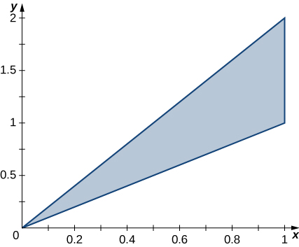
The triangular region RR with the vertices (0,0),(1,1),and(1,2)(0,0),(1,1),and(1,2) is shown in the following figure.

A triangle with corners at the origin, (1, 1), and (1, 2).
  1. Find a transformation T:S→R,T:S→R, T(u,v)=(x,y)=(au+bv,cu+dv),T(u,v)=(x,y)=(au+bv,cu+dv), where a,b,c,a,b,c, and dd are real numbers with ad−bc≠0ad−bc≠0 such that T−1(0,0)=(0,0),T−1(1,1)=(1,0),T−1(0,0)=(0,0),T−1(1,1)=(1,0), and T−1(1,2)=(0,1).T−1(1,2)=(0,1).
  2. Use the transformation TT to find the area A(R)A(R) of the region R.R.
389.

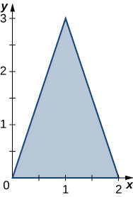
The triangular region RR with the vertices (0,0),(2,0),and(1,3)(0,0),(2,0),and(1,3) is shown in the following figure.

A triangle with corners at the origin, (2, 0), and (1, 3).
  1. Find a transformation T:S→R,T:S→R, T(u,v)=(x,y)=(au+bv,cu+dv),T(u,v)=(x,y)=(au+bv,cu+dv), where a,b,ca,b,c and dd are real numbers with ad−bc≠0ad−bc≠0 such that T−1(0,0)=(0,0),T−1(0,0)=(0,0), T−1(2,0)=(1,0),T−1(2,0)=(1,0), and T−1(1,3)=(0,1).T−1(1,3)=(0,1).
  2. Use the transformation TT to find the area A(R)A(R) of the region R.R.

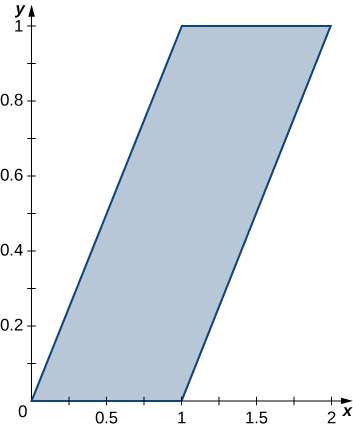
In the following exercises, use the transformation u=y−x,v=y,u=y−x,v=y, to evaluate the integrals on the parallelogram RR of vertices (0,0),(1,0),(2,1),and(1,1)(0,0),(1,0),(2,1),and(1,1) shown in the following figure.

A rhombus with corners at the origin, (1, 0), (1, 1), and (2, 1).
390.

∬ R ( y − x ) d A ∬ R ( y − x ) d A

391.

∬ R ( y 2 − x y ) d A ∬ R ( y 2 − x y ) d A

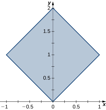
In the following exercises, use the transformation y−x=u,x+y=vy−x=u,x+y=v to evaluate the integrals on the square RR determined by the lines y=x,y=−x+2,y=x+2,y=x,y=−x+2,y=x+2, and y=−xy=−x shown in the following figure.

A square with side lengths square root of 2 rotated 45 degrees with one corner at the origin and another at (1, 1).
392.

∬ R e x + y d A ∬ R e x + y d A

393.

∬ R sin ( x − y ) d A ∬ R sin ( x − y ) d A

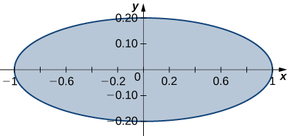
In the following exercises, use the transformation x=u,5y=vx=u,5y=v to evaluate the integrals on the region RR bounded by the ellipse x2+25y2=1x2+25y2=1 shown in the following figure.

An ellipse with center at the origin, major axis 2, and minor 0.4.
394.

∬ R x 2 + 25 y 2 d A ∬ R x 2 + 25 y 2 d A

395.

∬ R ( x 2 + 25 y 2 ) 2 d A ∬ R ( x 2 + 25 y 2 ) 2 d A

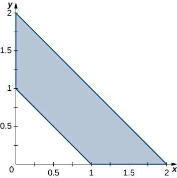
In the following exercises, use the transformation u=x+y,v=x−yu=x+y,v=x−y to evaluate the integrals on the trapezoidal region RR determined by the points (1,0),(2,0),(0,2),and(0,1)(1,0),(2,0),(0,2),and(0,1) shown in the following figure.

A trapezoid with corners at (1, 0), (0, 1), (0, 2), and (2, 0).
396.

∬ R ( x 2 − 2 x y + y 2 ) e x + y d A ∬ R ( x 2 − 2 x y + y 2 ) e x + y d A

397.

∬ R ( x 3 + 3 x 2 y + 3 x y 2 + y 3 ) d A ∬ R ( x 3 + 3 x 2 y + 3 x y 2 + y 3 ) d A

398.

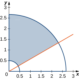
The circular annulus sector RR bounded by the circles 4x2+4y2=14x2+4y2=1 and 9x2+9y2=64,9x2+9y2=64, the line x=y3,x=y3, and the y-axisy-axis is shown in the following figure. Find a transformation TT from a rectangular region SS in the rθ-planerθ-plane to the region RR in the xy-plane.xy-plane. Graph S.S.

In the first quadrant, a section of an annulus described by an inner radius of 0.5, outer radius slightly more than 2.5, and center the origin. There is a line dividing this annulus that comes from approximately a 30 degree angle. The portion corresponding to 60 degrees is shaded.
399.

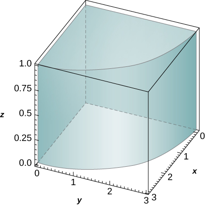
The solid RR bounded by the circular cylinder x2+y2=9x2+y2=9 and the planes z=0,z=1,z=0,z=1, x=0,andy=0x=0,andy=0 is shown in the following figure. Find a transformation TT from a cylindrical box SS in rθz-spacerθz-space to the solid RR in xyz-space.xyz-space.

A quarter of a cylinder with height 1 and radius 3. The center axis is the z axis.
400.

Show that ∬Rf(x23+y23)dA=2π15∫01f(ρ)ρdρ,∬Rf(x23+y23)dA=2π15∫01f(ρ)ρdρ, where ff is a continuous function on [0,1][0,1] and RR is the region bounded by the ellipse 5x2+3y2=15.5x2+3y2=15.

401.

Show that ∭Rf(16x2+4y2+z2)dV=π2∫01f(ρ)ρ2dρ,∭Rf(16x2+4y2+z2)dV=π2∫01f(ρ)ρ2dρ, where ff is a continuous function on [0,1][0,1] and RR is the region bounded by the ellipsoid 16x2+4y2+z2=1.16x2+4y2+z2=1.

402.

[T] Find the area of the region bounded by the curves xy=1,xy=3,y=2x,xy=1,xy=3,y=2x, and y=3xy=3x by using the transformation u=xyu=xy and v=yx.v=yx. Use a computer algebra system (CAS) to graph the boundary curves of the region R.R.

403.

[T] Find the area of the region bounded by the curves xy=2,xy=3,y=x,xy=2,xy=3,y=x, and y=2xy=2x by using the transformation u=xyu=xy and v=yx.v=yx.

404.

Evaluate the triple integral ∫01∫12∫zz+1(y+1)dxdydz∫01∫12∫zz+1(y+1)dxdydz by using the transformation u=x−z,u=x−z, v=3y,andw=z2.v=3y,andw=z2.

405.

Evaluate the triple integral ∫02∫46∫3z3z+2(5−4y)dxdzdy∫02∫46∫3z3z+2(5−4y)dxdzdy by using the transformation u=x−3z,v=4y,andw=z.u=x−3z,v=4y,andw=z.

406.

A transformation T:ℝ2→ℝ2,T(u,v)=(x,y)T:ℝ2→ℝ2,T(u,v)=(x,y) of the form x=au+bv,y=cu+dv,x=au+bv,y=cu+dv, where a,b,c,andda,b,c,andd are real numbers, is called linear. Show that a linear transformation for which ad−bc≠0ad−bc≠0 maps parallelograms to parallelograms.

407.

The transformation Tθ:ℝ2→ℝ2,Tθ(u,v)=(x,y),Tθ:ℝ2→ℝ2,Tθ(u,v)=(x,y), where x=ucosθ−vsinθ,x=ucosθ−vsinθ, y=usinθ+vcosθ,y=usinθ+vcosθ, is called a rotation of angle θ.θ. Show that the inverse transformation of TθTθ satisfies Tθ−1=T−θ,Tθ−1=T−θ, where T−θT−θ is the rotation of angle −θ.−θ.

408.

[T] Use the results of the previous exercise to find the region SS in the uv-planeuv-plane whose image through a rotation of angle π4π4 is the region RR enclosed by the ellipse x2+4y2=1.x2+4y2=1. Use a CAS to answer the following questions.

  1. Graph the region S.S.
  2. Evaluate the integral ∬Se−2uvdudv.∬Se−2uvdudv. Round your answer to two decimal places.
409.

[T] The transformations Ti:ℝ2→ℝ2,Ti:ℝ2→ℝ2, i=1,…,4,i=1,…,4, defined by T1(u,v)=(u,−v),T1(u,v)=(u,−v), T2(u,v)=(−u,v),T3(u,v)=(−u,−v),T2(u,v)=(−u,v),T3(u,v)=(−u,−v), and T4(u,v)=(v,u)T4(u,v)=(v,u) are called reflections about the x-axis,y-axis,x-axis,y-axis, origin, and the line y=x,y=x, respectively.

  1. Find the image of the region S={(u,v)|u2+v2−2u−4v+1≤0}S={(u,v)|u2+v2−2u−4v+1≤0} in the xy-planexy-plane through the transformation T1∘T2∘T3∘T4.T1∘T2∘T3∘T4.
  2. Use a CAS to graph the image of S.S.
  3. Evaluate the integral ∬Ssin(u2)dudv∬Ssin(u2)dudv by using a CAS. Round your answer to two decimal places.
410.

[T] The transformation Tk,1,1:ℝ3→ℝ3,Tk,1,1(u,v,w)=(x,y,z)Tk,1,1:ℝ3→ℝ3,Tk,1,1(u,v,w)=(x,y,z) of the form x=ku,x=ku, y=v,z=w,y=v,z=w, where k≠1k≠1 is a positive real number, is called a stretch if k>1k>1 and a compression if 0<k<10<k<1 in the x-direction.x-direction. Use a CAS to evaluate the integral ∭Se−(4x2+9y2+25z2)dxdydz∭Se−(4x2+9y2+25z2)dxdydz on the solid S={(x,y,z)|4x2+9y2+25z2≤1}S={(x,y,z)|4x2+9y2+25z2≤1} by considering the compression T2,3,5(u,v,w)=(x,y,z)T2,3,5(u,v,w)=(x,y,z) defined by x=u2,y=v3,x=u2,y=v3, and z=w5.z=w5. Round your answer to four decimal places.

411.

[T] The transformation Ta,0:ℝ2→ℝ2,Ta,0(u,v)=(u+av,v),Ta,0:ℝ2→ℝ2,Ta,0(u,v)=(u+av,v), where a≠0a≠0 is a real number, is called a shear in the x-direction.x-direction. The transformation, T0,b:ℝ2→ℝ2,T0,b(u,v)=(u,bu+v),T0,b:ℝ2→ℝ2,T0,b(u,v)=(u,bu+v), where b≠0b≠0 is a real number, is called a shear in the y-direction.y-direction.

  1. Find transformations T0,2∘T3,0.T0,2∘T3,0.
  2. Find the image RR of the trapezoidal region SS bounded by u=0,v=0,v=1,u=0,v=0,v=1, and v=2−uv=2−u through the transformation T0,2∘T3,0.T0,2∘T3,0.
  3. Use a CAS to graph the image RR in the xy-plane.xy-plane.
  4. Find the area of the region RR by using the area of region S.S.
412.

Use the transformation, x=au,y=av,z=cwx=au,y=av,z=cw and spherical coordinates to show that the volume of a region bounded by the spheroid x2+y2a2+z2c2=1x2+y2a2+z2c2=1 is 4πa2c3.4πa2c3.

413.

Find the volume of a football whose shape is a spheroid x2+y2a2+z2c2=1x2+y2a2+z2c2=1 whose length from tip to tip is 1111 inches and circumference at the center is 2222 inches. Round your answer to two decimal places.

414.

[T] Lamé ovals (or superellipses) are plane curves of equations (xa)n+(yb)n=1,(xa)n+(yb)n=1, where a, b, and n are positive real numbers.

  1. Use a CAS to graph the regions RR bounded by Lamé ovals for a=1,b=2,n=4a=1,b=2,n=4 and n=6,n=6, respectively.
  2. Find the transformations that map the region RR bounded by the Lamé oval x4+y4=1,x4+y4=1, also called a squircle and graphed in the following figure, into the unit disk.
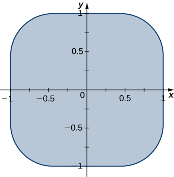
    A square of side length 2 with rounded corners.
  3. Use a CAS to find an approximation of the area A(R)A(R) of the region RR bounded by x4+y4=1.x4+y4=1. Round your answer to two decimal places.
415.

[T] Lamé ovals have been consistently used by designers and architects. For instance, Gerald Robinson, a Canadian architect, has designed a parking garage in a shopping center in Peterborough, Ontario, in the shape of a superellipse of the equation (xa)n+(yb)n=1(xa)n+(yb)n=1 with ab=97ab=97 and n=e.n=e. Use a CAS to find an approximation of the area of the parking garage in the case a=900a=900 yards, b=700b=700 yards, and n=2.72n=2.72.