Partial Fractions - Calculus Volume 2

3.4 Partial Fractions

Learning Objectives

3.4.1 Integrate a rational function using the method of partial fractions.
3.4.2 Recognize simple linear factors in a rational function.
3.4.3 Recognize repeated linear factors in a rational function.
3.4.4 Recognize quadratic factors in a rational function.

We have seen some techniques that allow us to integrate specific rational functions. For example, we know that

\int \frac{d u}{u} = ln | u | + C and \int \frac{d u}{u^{2} + a^{2}} = \frac{1}{a} {tan}^{−1} (\frac{u}{a}) + C .

However, we do not yet have a technique that allows us to tackle arbitrary quotients of this type. Thus, it is not immediately obvious how to go about evaluating $\int \frac{3 x}{x^{2} - x - 2} d x .$ However, we know from material previously developed that

\int (\frac{1}{x + 1} + \frac{2}{x - 2}) d x = ln | x + 1 | + 2 ln | x - 2 | + C .

In fact, by getting a common denominator, we see that

\frac{1}{x + 1} + \frac{2}{x - 2} = \frac{3 x}{x^{2} - x - 2} .

Consequently,

\int \frac{3 x}{x^{2} - x - 2} d x = \int (\frac{1}{x + 1} + \frac{2}{x - 2}) d x .

In this section, we examine the method of partial fraction decomposition, which allows us to decompose rational functions into sums of simpler, more easily integrated rational functions. Using this method, we can rewrite an expression such as: $\frac{3 x}{x^{2} - x - 2}$ as an expression such as $\frac{1}{x + 1} + \frac{2}{x - 2} .$

The key to the method of partial fraction decomposition is being able to anticipate the form that the decomposition of a rational function will take. As we shall see, this form is both predictable and highly dependent on the factorization of the denominator of the rational function. It is also extremely important to keep in mind that partial fraction decomposition can be applied to a rational function $\frac{P (x)}{Q (x)}$ only if $deg (P (x)) < deg (Q (x)) .$ In the case when $deg (P (x)) \geq deg (Q (x)),$ we must first perform long division to rewrite the quotient $\frac{P (x)}{Q (x)}$ in the form $A (x) + \frac{R (x)}{Q (x)},$ where $deg (R (x)) < deg (Q (x)) .$ We then do a partial fraction decomposition on $\frac{R (x)}{Q (x)} .$ The following example, although not requiring partial fraction decomposition, illustrates our approach to integrals of rational functions of the form $\int \frac{P (x)}{Q (x)} d x,$ where $deg (P (x)) \geq deg (Q (x)) .$

Example 3.28

Integrating $\int \frac{P (x)}{Q (x)} d x,$ where $deg (P (x)) \geq deg (Q (x))$

Evaluate $\int \frac{x^{2} + 3 x + 5}{x + 1} d x .$

Solution

Since $deg (x^{2} + 3 x + 5) \geq deg (x + 1),$ we perform long division to obtain

\frac{x^{2} + 3 x + 5}{x + 1} = x + 2 + \frac{3}{x + 1} .

Thus,

\begin{matrix} \int \frac{x^{2} + 3 x + 5}{x + 1} d x & = \int (x + 2 + \frac{3}{x + 1}) d x \\ = \frac{1}{2} x^{2} + 2 x + 3 ln | x + 1 | + C . \end{matrix}

Media

Visit this website for a review of long division of polynomials.

Checkpoint 3.17

Evaluate $\int \frac{x - 3}{x + 2} d x .$

To integrate $\int \frac{P (x)}{Q (x)} d x,$ where $deg (P (x)) < deg (Q (x)),$ we must begin by factoring $Q (x) .$

Nonrepeated Linear Factors

If $Q (x)$ can be factored as $(a_{1} x + b_{1}) (a_{2} x + b_{2}) … (a_{n} x + b_{n}),$ where each linear factor is distinct, then it is possible to find constants $A_{1}, A_{2},… A_{n}$ satisfying

\frac{P (x)}{Q (x)} = \frac{A_{1}}{a_{1} x + b_{1}} + \frac{A_{2}}{a_{2} x + b_{2}} + \dots + \frac{A_{n}}{a_{n} x + b_{n}} .

The proof that such constants exist is beyond the scope of this course.

In this next example, we see how to use partial fractions to integrate a rational function of this type.

Example 3.29

Partial Fractions with Nonrepeated Linear Factors

Evaluate $\int \frac{3 x + 2}{x^{3} - x^{2} - 2 x} d x .$

Solution

Since $deg (3 x + 2) < deg (x^{3} - x^{2} - 2 x),$ we begin by factoring the denominator of $\frac{3 x + 2}{x^{3} - x^{2} - 2 x} .$ We can see that $x^{3} - x^{2} - 2 x = x (x - 2) (x + 1) .$ Thus, there are constants $A,$ $B,$ and $C$ satisfying

\frac{3 x + 2}{x (x - 2) (x + 1)} = \frac{A}{x} + \frac{B}{x - 2} + \frac{C}{x + 1} .

We must now find these constants. To do so, we begin by getting a common denominator on the right. Thus,

\frac{3 x + 2}{x (x - 2) (x + 1)} = \frac{A (x - 2) (x + 1) + B x (x + 1) + C x (x - 2)}{x (x - 2) (x + 1)} .

Now, we set the numerators equal to each other, obtaining

3 x + 2 = A (x - 2) (x + 1) + B x (x + 1) + C x (x - 2) .

(3.8)

There are two different strategies for finding the coefficients $A,$ $B,$ and $C .$ We refer to these as the method of equating coefficients and the method of strategic substitution.

Rule: Method of Equating Coefficients

Rewrite Equation 3.8 in the form

3 x + 2 = (A + B + C) x^{2} + (− A + B - 2 C) x + (−2 A) .

Equating coefficients produces the system of equations

\begin{matrix} A + B + C & = & 0 \\ - A + B - 2 C & = & 3 \\ - 2 A & = & 2. \end{matrix}

To solve this system, we first observe that $−2 A = 2 \Rightarrow A = −1 .$ Substituting this value into the first two equations gives us the system

\begin{matrix} B + C & = & 1 \\ B - 2 C & = & 2. \end{matrix}

Multiplying the second equation by $−1$ and adding the resulting equation to the first produces

−3 C = 1,

which in turn implies that $C = - \frac{1}{3} .$ Substituting this value into the equation $B + C = 1$ yields $B = \frac{4}{3} .$ Thus, solving these equations yields $A = −1,$ $B = \frac{4}{3},$ and $C = - \frac{1}{3} .$

It is important to note that the system produced by this method is consistent if and only if we have set up the decomposition correctly. If the system is inconsistent, there is an error in our decomposition.

Rule: Method of Strategic Substitution

The method of strategic substitution is based on the assumption that we have set up the decomposition correctly. If the decomposition is set up correctly, then there must be values of $A,$ $B,$ and $C$ that satisfy Equation 3.8 for all values of $x .$ That is, this equation must be true for any value of $x$ we care to substitute into it. Therefore, by choosing values of $x$ carefully and substituting them into the equation, we may find $A,$ $B,$ and $C$ easily. For example, if we substitute $x = 0,$ the equation reduces to $2 = A (−2) (1) .$ Solving for $A$ yields $A = −1 .$ Next, by substituting $x = 2,$ the equation reduces to $8 = B (2) (3),$ or equivalently $B = 4 / 3 .$ Last, we substitute $x = −1$ into the equation and obtain $−1 = C (−1) (−3) .$ Solving, we have $C = - \frac{1}{3} .$

It is important to keep in mind that if we attempt to use this method with a decomposition that has not been set up correctly, we are still able to find values for the constants, but these constants are meaningless. If we do opt to use the method of strategic substitution, then it is a good idea to check the result by recombining the terms algebraically.

Now that we have the values of $A,$ $B,$ and $C,$ we rewrite the original integral:

\int \frac{3 x + 2}{x^{3} - x^{2} - 2 x} d x = \int (− \frac{1}{x} + \frac{4}{3} \cdot \frac{1}{(x - 2)} - \frac{1}{3} \cdot \frac{1}{(x + 1)}) d x .

Evaluating the integral gives us

\int \frac{3 x + 2}{x^{3} - x^{2} - 2 x} d x = − ln | x | + \frac{4}{3} ln | x - 2 | - \frac{1}{3} ln | x + 1 | + C .

In the next example, we integrate a rational function in which the degree of the numerator is not less than the degree of the denominator.

Example 3.30

Dividing before Applying Partial Fractions

Evaluate $\int \frac{x^{2} + 3 x + 1}{x^{2} - 4} d x .$

Solution

Since $degree (x^{2} + 3 x + 1) \geq degree (x^{2} - 4),$ we must perform long division of polynomials. This results in

\frac{x^{2} + 3 x + 1}{x^{2} - 4} = 1 + \frac{3 x + 5}{x^{2} - 4} .

Next, we perform partial fraction decomposition on $\frac{3 x + 5}{x^{2} - 4} = \frac{3 x + 5}{(x + 2) (x - 2)} .$ We have

\frac{3 x + 5}{(x - 2) (x + 2)} = \frac{A}{x - 2} + \frac{B}{x + 2} .

Thus,

3 x + 5 = A (x + 2) + B (x - 2) .

Solving for $A$ and $B$ using either method, we obtain $A = 11 / 4$ and $B = 1 / 4 .$

Rewriting the original integral, we have

\int \frac{x^{2} + 3 x + 1}{x^{2} - 4} d x = \int (1 + \frac{11}{4} \cdot \frac{1}{x - 2} + \frac{1}{4} \cdot \frac{1}{x + 2}) d x .

Evaluating the integral produces

\int \frac{x^{2} + 3 x + 1}{x^{2} - 4} d x = x + \frac{11}{4} ln | x - 2 | + \frac{1}{4} ln | x + 2 | + C .

As we see in the next example, it may be possible to apply the technique of partial fraction decomposition to a nonrational function. The trick is to convert the nonrational function to a rational function through a substitution.

Example 3.31

Applying Partial Fractions after a Substitution

Evaluate $\int \frac{cos x}{{sin}^{2} x - sin x} d x .$

Solution

Let’s begin by letting $u = sin x .$ Consequently, $d u = cos x d x .$ After making these substitutions, we have

\int \frac{cos x}{{sin}^{2} x - sin x} d x = \int \frac{d u}{u^{2} - u} = \int \frac{d u}{u (u - 1)} .

Applying partial fraction decomposition to $1 / u (u - 1)$ gives $\frac{1}{u (u - 1)} = - \frac{1}{u} + \frac{1}{u - 1} .$

Thus,

\begin{matrix} \int \frac{cos x}{{sin}^{2} x - sin x} d x & = − ln | u | + ln | u - 1 | + C \\ = − ln | sin x | + ln | sin x - 1 | + C . \end{matrix}

Checkpoint 3.18

Evaluate $\int \frac{x + 1}{(x + 3) (x - 2)} d x .$

Repeated Linear Factors

For some applications, we need to integrate rational expressions that have denominators with repeated linear factors—that is, rational functions with at least one factor of the form ${(a x + b)}^{n},$ where $n$ is a positive integer greater than or equal to $2 .$ If the denominator contains the repeated linear factor ${(a x + b)}^{n},$ then the decomposition must contain

\frac{A_{1}}{a x + b} + \frac{A_{2}}{{(a x + b)}^{2}} + \dots + \frac{A_{n}}{{(a x + b)}^{n}} .

As we see in our next example, the basic technique used for solving for the coefficients is the same, but it requires more algebra to determine the numerators of the partial fractions.

Example 3.32

Partial Fractions with Repeated Linear Factors

Evaluate $\int \frac{x - 2}{{(2 x - 1)}^{2} (x - 1)} d x .$

Solution

We have $degree (x - 2) < degree ({(2 x - 1)}^{2} (x - 1)),$ so we can proceed with the decomposition. Since ${(2 x - 1)}^{2}$ is a repeated linear factor, include $\frac{A}{2 x - 1} + \frac{B}{{(2 x - 1)}^{2}}$ in the decomposition. Thus,

\frac{x - 2}{{(2 x - 1)}^{2} (x - 1)} = \frac{A}{2 x - 1} + \frac{B}{{(2 x - 1)}^{2}} + \frac{C}{x - 1} .

After getting a common denominator and equating the numerators, we have

x - 2 = A (2 x - 1) (x - 1) + B (x - 1) + C {(2 x - 1)}^{2} .

(3.9)

We then use the method of equating coefficients to find the values of $A,$ $B,$ and $C .$

x - 2 = (2 A + 4 C) x^{2} + (−3 A + B - 4 C) x + (A - B + C) .

Equating coefficients yields $2 A + 4 C = 0,$ $−3 A + B - 4 C = 1,$ and $A - B + C = −2 .$ Solving this system yields $A = 2,$ $B = 3,$ and $C = −1 .$

Alternatively, we can use the method of strategic substitution. In this case, substituting $x = 1$ and $x = 1 / 2$ into Equation 3.9 easily produces the values $B = 3$ and $C = −1 .$ At this point, it may seem that we have run out of good choices for $x,$ however, since we already have values for $B$ and $C,$ we can substitute in these values and choose any value for $x$ not previously used. The value $x = 0$ is a good option. In this case, we obtain the equation $−2 = A (−1) (−1) + 3 (−1) + (−1) {(−1)}^{2}$ or, equivalently, $A = 2 .$

Now that we have the values for $A,$ $B,$ and $C,$ we rewrite the original integral and evaluate it:

\begin{matrix} \int \frac{x - 2}{{(2 x - 1)}^{2} (x - 1)} d x & = \int (\frac{2}{2 x - 1} + \frac{3}{{(2 x - 1)}^{2}} - \frac{1}{x - 1}) d x \\ = ln | 2 x - 1 | - \frac{3}{2 (2 x - 1)} - ln | x - 1 | + C . \end{matrix}

Checkpoint 3.19

Set up the partial fraction decomposition for $\int \frac{x + 2}{{(x + 3)}^{3} {(x - 4)}^{2}} d x .$ (Do not solve for the coefficients or complete the integration.)

The General Method

Now that we are beginning to get the idea of how the technique of partial fraction decomposition works, let’s outline the basic method in the following problem-solving strategy.

Problem-Solving Strategy

Partial Fraction Decomposition

To decompose the rational function $P (x) / Q (x),$ use the following steps:

Make sure that $degree (P (x)) < degree (Q (x)) .$ If not, perform long division of polynomials.
Factor $Q (x)$ into the product of linear and irreducible quadratic factors. An irreducible quadratic is a quadratic that has no real zeros.
Assuming that deg(P(x))<deg(Q(x)),deg(P(x))<deg(Q(x)), the factors of Q(x)Q(x) determine the form of the decomposition of P(x)/Q(x).P(x)/Q(x).
1. If $Q (x)$ can be factored as $(a_{1} x + b_{1}) (a_{2} x + b_{2}) … (a_{n} x + b_{n}),$ where each linear factor is distinct, then it is possible to find constants $A_{1}, A_{2}, . . . A_{n}$ satisfying
  
  $\frac{P (x)}{Q (x)} = \frac{A_{1}}{a_{1} x + b_{1}} + \frac{A_{2}}{a_{2} x + b_{2}} + \dots + \frac{A_{n}}{a_{n} x + b_{n}} .$
2. If $Q (x)$ contains the repeated linear factor ${(a x + b)}^{n},$ then the decomposition must contain
  
  $\frac{A_{1}}{a x + b} + \frac{A_{2}}{{(a x + b)}^{2}} + \dots + \frac{A_{n}}{{(a x + b)}^{n}} .$
3. For each irreducible quadratic factor $a x^{2} + b x + c$ that $Q (x)$ contains, the decomposition must include
  
  $\frac{A x + B}{a x^{2} + b x + c} .$
4. For each repeated irreducible quadratic factor ${(a x^{2} + b x + c)}^{n},$ the decomposition must include
  
  $\frac{A_{1} x + B_{1}}{a x^{2} + b x + c} + \frac{A_{2} x + B_{2}}{{(a x^{2} + b x + c)}^{2}} + \dots + \frac{A_{n} x + B_{n}}{{(a x^{2} + b x + c)}^{n}} .$
5. After the appropriate decomposition is determined, solve for the constants.
6. Last, rewrite the integral in its decomposed form and evaluate it using previously developed techniques or integration formulas.

Simple Quadratic Factors

Now let’s look at integrating a rational expression in which the denominator contains an irreducible quadratic factor. Recall that the quadratic $a x^{2} + b x + c$ is irreducible if $a x^{2} + b x + c = 0$ has no real zeros—that is, if $b^{2} - 4 a c < 0 .$

Example 3.33

Rational Expressions with an Irreducible Quadratic Factor

Evaluate $\int \frac{2 x - 3}{x^{3} + x} d x .$

Solution

Since $deg (2 x - 3) < deg (x^{3} + x),$ factor the denominator and proceed with partial fraction decomposition. Since $x^{3} + x = x (x^{2} + 1)$ contains the irreducible quadratic factor $x^{2} + 1,$ include $\frac{A x + B}{x^{2} + 1}$ as part of the decomposition, along with $\frac{C}{x}$ for the linear term $x .$ Thus, the decomposition has the form

\frac{2 x - 3}{x (x^{2} + 1)} = \frac{A x + B}{x^{2} + 1} + \frac{C}{x} .

After getting a common denominator and equating the numerators, we obtain the equation

2 x - 3 = (A x + B) x + C (x^{2} + 1) .

Solving for $A, B,$ and $C,$ we get $A = 3,$ $B = 2,$ and $C = −3 .$

Thus,

\frac{2 x - 3}{x^{3} + x} = \frac{3 x + 2}{x^{2} + 1} - \frac{3}{x} .

Substituting back into the integral, we obtain

\begin{matrix} \int \frac{2 x - 3}{x^{3} + x} d x & = \int (\frac{3 x + 2}{x^{2} + 1} - \frac{3}{x}) d x \\ = 3 \int \frac{x}{x^{2} + 1} d x + 2 \int \frac{1}{x^{2} + 1} d x - 3 \int \frac{1}{x} d x & Split up the integral. \\ = \frac{3}{2} ln | x^{2} + 1 | + 2 {tan}^{−1} x - 3 ln | x | + C . & Evaluate each integral. \end{matrix}

Note: We may rewrite $ln | x^{2} + 1 | = ln (x^{2} + 1),$ if we wish to do so, since $x^{2} + 1 > 0 .$

Example 3.34

Partial Fractions with an Irreducible Quadratic Factor

Evaluate $\int \frac{d x}{x^{3} - 8} .$

Solution

We can start by factoring $x^{3} - 8 = (x - 2) (x^{2} + 2 x + 4) .$ We see that the quadratic factor $x^{2} + 2 x + 4$ is irreducible since $2^{2} - 4 (1) (4) = −12 < 0 .$ Using the decomposition described in the problem-solving strategy, we get

\frac{1}{(x - 2) (x^{2} + 2 x + 4)} = \frac{A}{x - 2} + \frac{B x + C}{x^{2} + 2 x + 4} .

After obtaining a common denominator and equating the numerators, this becomes

1 = A (x^{2} + 2 x + 4) + (B x + C) (x - 2) .

Applying either method, we get $A = \frac{1}{12}, B = - \frac{1}{12}, and C = - \frac{1}{3} .$

Rewriting $\int \frac{d x}{x^{3} - 8},$ we have

\int \frac{d x}{x^{3} - 8} = \frac{1}{12} \int \frac{1}{x - 2} d x - \frac{1}{12} \int \frac{x + 4}{x^{2} + 2 x + 4} d x .

We can see that

$\int \frac{1}{x - 2} d x = ln | x - 2 | + C,$ but $\int \frac{x + 4}{x^{2} + 2 x + 4} d x$ requires a bit more effort. Let’s begin by completing the square on $x^{2} + 2 x + 4$ to obtain

x^{2} + 2 x + 4 = {(x + 1)}^{2} + 3 .

By letting $u = x + 1$ and consequently $d u = d x,$ we see that

\begin{matrix} \int \frac{x + 4}{x^{2} + 2 x + 4} d x & = \int \frac{x + 4}{{(x + 1)}^{2} + 3} d x & \begin{matrix} Complete the square on the \\ denominator. \end{matrix} \\ = \int \frac{u + 3}{u^{2} + 3} d u & \begin{matrix} Substitute u = x + 1, x = u - 1, \\ and d u = d x . \end{matrix} \\ = \int \frac{u}{u^{2} + 3} d u + \int \frac{3}{u^{2} + 3} d u & Split the numerator apart. \\ = \frac{1}{2} ln | u^{2} + 3 | + \frac{3}{\sqrt{3}} {tan}^{−1} \frac{u}{\sqrt{3}} + C & Evaluate each integral. \\ = \frac{1}{2} ln | x^{2} + 2 x + 4 | + \sqrt{3} {tan}^{−1} (\frac{x + 1}{\sqrt{3}}) + C . & \begin{matrix} Rewrite in terms of x and \\ simplify. \end{matrix} \end{matrix}

Substituting back into the original integral and simplifying gives

\int^{​} \frac{d x}{x^{3} - 8} = \frac{1}{12} ln | x - 2 | - \frac{1}{24} ln | x^{2} + 2 x + 4 | - \frac{\sqrt{3}}{12} {tan}^{−1} (\frac{x + 1}{\sqrt{3}}) + C .

Here again, we can drop the absolute value if we wish to do so, since $x^{2} + 2 x + 4 > 0$ for all $x .$

Example 3.35

Finding a Volume

Find the volume of the solid of revolution obtained by revolving the region enclosed by the graph of $f (x) = \frac{x^{2}}{{(x^{2} + 1)}^{2}}$ and the x-axis over the interval $[0, 1]$ about the y-axis.

Solution

Let’s begin by sketching the region to be revolved (see Figure 3.11). From the sketch, we see that the shell method is a good choice for solving this problem.

This figure is the graph of the function f(x) = x^2/(x^2+1)^2. It is a curve above the x-axis. It is decreasing in the second quadrant, intersects at the origin, and increases in the first quadrant. Between x = 0 and x = 1, there is shaded area under the curve.

Figure 3.11 We can use the shell method to find the volume of revolution obtained by revolving the region shown about the y-axis.

The volume is given by

V = 2 π \int_{0}^{1} x \cdot \frac{x^{2}}{{(x^{2} + 1)}^{2}} d x = 2 π \int_{0}^{1} \frac{x^{3}}{{(x^{2} + 1)}^{2}} d x .

Since $deg ({(x^{2} + 1)}^{2}) = 4 > 3 = deg (x^{3}),$ we can proceed with partial fraction decomposition. Note that ${(x^{2} + 1)}^{2}$ is a repeated irreducible quadratic. Using the decomposition described in the problem-solving strategy, we get

\frac{x^{3}}{{(x^{2} + 1)}^{2}} = \frac{A x + B}{x^{2} + 1} + \frac{C x + D}{{(x^{2} + 1)}^{2}} .

Finding a common denominator and equating the numerators gives

x^{3} = (A x + B) (x^{2} + 1) + C x + D .

Solving, we obtain $A = 1,$ $B = 0,$ $C = −1,$ and $D = 0 .$ Substituting back into the integral, we have

\begin{matrix} V & = 2 π \int_{0}^{1} \frac{x^{3}}{{(x^{2} + 1)}^{2}} d x \\ = 2 π \int_{0}^{1} (\frac{x}{x^{2} + 1} - \frac{x}{{(x^{2} + 1)}^{2}}) d x \\ = 2 π (\frac{1}{2} ln (x^{2} + 1) + \frac{1}{2} \cdot \frac{1}{x^{2} + 1}) |_{\begin{matrix} 0 \end{matrix}}^{\begin{matrix} 1 \end{matrix}} \\ = π (ln 2 - \frac{1}{2}) . \end{matrix}

Checkpoint 3.20

Set up the partial fraction decomposition for $\int \frac{x^{2} + 3 x + 1}{(x + 2) {(x - 3)}^{2} {(x^{2} + 4)}^{2}} d x .$

Section 3.4 Exercises

Express the rational function as a sum or difference of two simpler rational expressions.

182.

$\frac{1}{(x - 3) (x - 2)}$

183.

$\frac{x^{2} + 1}{x (x + 1) (x + 2)}$

184.

$\frac{1}{x^{3} - x}$

185.

$\frac{3 x + 1}{x^{2}}$

186.

$\frac{3 x^{2}}{x^{2} + 1}$ (Hint: Use long division first.)

187.

$\frac{2 x^{4}}{x^{2} - 2 x}$

188.

$\frac{1}{(x - 1) (x^{2} + 1)}$

189.

$\frac{1}{x^{2} (x - 1)}$

190.

$\frac{x}{x^{2} - 4}$

191.

$\frac{1}{x (x - 1) (x - 2) (x - 3)}$

192.

$\frac{1}{x^{4} - 1} = \frac{1}{(x + 1) (x - 1) (x^{2} + 1)}$

193.

$\frac{3 x^{2}}{x^{3} - 1} = \frac{3 x^{2}}{(x - 1) (x^{2} + x + 1)}$

194.

$\frac{2 x}{{(x + 2)}^{2}}$

195.

$\frac{3 x^{4} + x^{3} + 20 x^{2} + 3 x + 31}{(x + 1) {(x^{2} + 4)}^{2}}$

Use the method of partial fractions to evaluate each of the following integrals.

196.

$\int \frac{d x}{(x - 3) (x - 2)}$

197.

$\int \frac{3 x}{x^{2} + 2 x - 8} d x$

198.

$\int \frac{d x}{x^{3} - x}$

199.

$\int \frac{x}{x^{2} - 4} d x$

200.

$\int \frac{d x}{x (x - 1) (x - 2) (x - 3)}$

201.

$\int \frac{2 x^{2} + 4 x + 22}{x^{2} + 2 x + 10} d x$

202.

$\int \frac{d x}{x^{2} - 5 x + 6}$

203.

$\int \frac{2 - x}{x^{2} + x} d x$

204.

$\int \frac{2}{x^{2} - x - 6} d x$

205.

$\int \frac{d x}{x^{3} - 2 x^{2} - 4 x + 8}$

206.

$\int \frac{d x}{x^{4} - 10 x^{2} + 9}$

Evaluate the following integrals, which have irreducible quadratic factors.

207.

$\int \frac{2}{(x - 4) (x^{2} + 2 x + 6)} d x$

208.

$\int \frac{x^{2}}{x^{3} - x^{2} + 4 x - 4} d x$

209.

$\int \frac{x^{3} + 6 x^{2} + 3 x + 6}{x^{3} + 2 x^{2}} d x$

210.

$\int \frac{x}{(x - 1) {(x^{2} + 2 x + 2)}^{2}} d x$

Use the method of partial fractions to evaluate the following integrals.

211.

$\int \frac{3 x + 4}{(x^{2} + 4) (3 - x)} d x$

212.

$\int \frac{2}{{(x + 2)}^{2} (2 - x)} d x$

213.

$\int \frac{3 x + 4}{x^{3} - 2 x - 4} d x$ (Hint: Use the rational root theorem.)

Use substitution to convert the integrals to integrals of rational functions. Then use partial fractions to evaluate the integrals.

214.

$\int_{0}^{1} \frac{e^{x}}{36 - e^{2 x}} d x$ (Give the exact answer and the decimal equivalent. Round to five decimal places.)

215.

$\int \frac{e^{x}}{e^{2 x} - e^{x}} d x$

216.

$\int \frac{sin x d x}{1 - {cos}^{2} x}$

217.

$\int \frac{sin x}{{cos}^{2} x + cos x - 6} d x$

218.

$\int \frac{1 - \sqrt{x}}{1 + \sqrt{x}} d x$

219.

$\int \frac{d t}{{(e^{t} - e^{− t})}^{2}}$

220.

$\int \frac{1 + e^{x}}{1 - e^{x}} d x$

221.

$\int \frac{d x}{1 + \sqrt{x + 1}}$

222.

$\int \frac{d x}{\sqrt{x} + \sqrt[4]{x}}$

223.

$\int \frac{cos x}{sin x (1 - sin x)} d x$

224.

$\int \frac{e^{x}}{{(e^{2 x} - 4)}^{2}} d x$

225.

$\int_{1}^{2} \frac{1}{x^{2} \sqrt{4 - x^{2}}} d x$

226.

$\int \frac{1}{2 + e^{− x}} d x$

227.

$\int \frac{1}{1 + e^{x}} d x$

Use the given substitution to convert the integral to an integral of a rational function, then evaluate.

228.

$\int \frac{1}{t - \sqrt[3]{t}} d t t = x^{3}$

229.

$\int \frac{1}{\sqrt{x} + \sqrt[3]{x}} d x; x = u^{6}$

230.

Graph the curve $y = \frac{x}{1 + x}$ over the interval $[0, 5] .$ Then, find the area of the region bounded by the curve, the x-axis, and the line $x = 4 .$

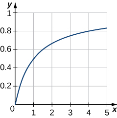
This figure is a graph of the function y = x/(1 + x). The graph is only in the first quadrant. It begins at the origin and increases into the first quadrant. The curve stops at x = 5.

231.

Find the volume of the solid generated when the region bounded by $y = 1 / \sqrt{x (3 - x)},$ $y = 0,$ $x = 1,$ and $x = 2$ is revolved about the x-axis.

232.

The velocity of a particle moving along a line is a function of time given by $v (t) = \frac{88 t^{2}}{t^{2} + 1} .$ Find the distance that the particle has traveled after $t = 5$ sec.

Solve the initial-value problem for x as a function of t.

233.

$(t^{2} - 7 t + 12) \frac{d x}{d t} = 1, (t > 4, x (5) = 0)$

234.

$(t + 5) \frac{d x}{d t} = x^{2} + 1, t > − 5, x (1) = tan 1$

235.

$(2 t^{3} - 2 t^{2} + t - 1) \frac{d x}{d t} = 3, x (2) = 0$

236.

Find the x-coordinate of the centroid of the area bounded by

$y (x^{2} - 9) = 1,$ $y = 0, x = 4, and x = 5 .$ (Round the answer to two decimal places.)

237.

Find the volume generated by revolving the area bounded by $y = \frac{1}{x^{3} + 7 x^{2} + 6 x}, x = 1, x = 7, and y = 0$ about the y-axis.

238.

Find the area bounded by $y = \frac{x - 12}{x^{2} - 8 x - 20},$ $y = 0, x = 2, and x = 4 .$ (Round the answer to the nearest hundredth.)

239.

Evaluate the integral $\int \frac{d x}{x^{3} + 1} .$

For the following problems, use the substitutions $tan (\frac{x}{2}) = t,$ $d x = \frac{2}{1 + t^{2}} d t,$ $sin x = \frac{2 t}{1 + t^{2}},$ and $cos x = \frac{1 - t^{2}}{1 + t^{2}} .$

240.

$\int \frac{d x}{3 - 5 sin x}$

241.

Find the area under the curve $y = \frac{1}{1 + sin x}$ between $x = 0$ and $x = π .$ (Assume the dimensions are in inches.)

242.

Given $tan (\frac{x}{2}) = t,$ derive the formulas $d x = \frac{2}{1 + t^{2}} d t,$ $sin x = \frac{2 t}{1 + t^{2}},$ and $cos x = \frac{1 - t^{2}}{1 + t^{2}} .$

243.

Evaluate $\int \frac{\sqrt[3]{x - 8}}{x} d x .$

3.4 Partial Fractions

Learning Objectives

Example 3.28

Integrating ∫P(x)Q(x)dx,∫P(x)Q(x)dx, where deg(P(x))≥deg(Q(x))deg(P(x))≥deg(Q(x))

Solution

Media

Checkpoint 3.17

Nonrepeated Linear Factors

Example 3.29

Partial Fractions with Nonrepeated Linear Factors

Solution

Rule: Method of Equating Coefficients

Rule: Method of Strategic Substitution

Example 3.30

Dividing before Applying Partial Fractions

Solution

Example 3.31

Applying Partial Fractions after a Substitution

Solution

Checkpoint 3.18

Repeated Linear Factors

Example 3.32

Partial Fractions with Repeated Linear Factors

Solution

Checkpoint 3.19

The General Method

Problem-Solving Strategy

Partial Fraction Decomposition

Simple Quadratic Factors

Example 3.33

Rational Expressions with an Irreducible Quadratic Factor

Solution

Example 3.34

Partial Fractions with an Irreducible Quadratic Factor

Solution

Example 3.35

Finding a Volume

Solution

Checkpoint 3.20

Section 3.4 Exercises

Integrating $\int \frac{P (x)}{Q (x)} d x,$ where $deg (P (x)) \geq deg (Q (x))$